Back to basics: Scaling train and test samples.

The importance of scaling

Scaling data is essential before applying a lot of Machine Learning techniques. For example, distance-based methods such as K-Nearest Neighbors, Principal Component Analysis or Support-Vector Machines will artificially attribute a great importance to a given feature if its range is extremely broad. As a consequence, these kind of algorithms require scaling to work properly. Although not absolutely necessary, scaling and specifically normalizing helps a lot with the convergence of gradient descent [1]. Hence it is generally recommended for Deep Learning. On the contrary, tree-based methods such as Random Forest or XGBoost do not require the input features to be scaled.

Today, we will only consider the two main ways of scaling, i.e standardization, a.k.a Z-score normalization and normalization, a.k.a Min-Max scaling. The standardized version of the numerical feature $X$ is: $$\tilde{X} := \frac{X - \overline{X}}{\hat{\sigma}}$$ where $\overline{X}$ is the estimated mean of $X$ and $\hat{\sigma}$ its estimated standard deviation. The point of this transformation is that $\tilde{X}$ has an estimated mean equal to 0 and an estimated standard deviation equal to 1.

On the other hand, normalization consists in the transformation: $$\tilde{X} := \frac{X - min(X)}{max(X) - min(X)}$$ Consequently, $\tilde{X} \in [0;1]$.

Scaling can be tricky

In his excellent blog post, Sebastian Raschka explains why the only one way to properly split and scale a dataset is the following one :

1. Train-test split the data
2. Scale the train sample
3. Scale the test sample with the training parameters

Any other method (scaling then splitting or scaling each sample with its own parameters for example) is wrong because it makes use of information extracted from the test sample to build the model afterwards. Sebastian gives extreme examples to illustrate this in his post. Although improper scaling may have minor consequences when working with a large dataset, it can seriously diminish the performance of a given model if only a few observations are available.

Programmatically speaking, splitting and scaling a dataset using the method presented above can be a little bit more troublesome than just scaling a set of observations by itself. Let us see how to proceed in a variety of frameworks. As an example, we will work on a dataset composed of three independent features:

• $X \sim \mathcal{N}(\mu = 2, \sigma = 2)$
• $Y \sim \mathcal{C}(x_0 = 0, \gamma = 1)$
• $Z \sim \mathcal{U}(a = 5, b = 10)$

Where the letters $\mathcal{N}$, $\mathcal{C}$ and $\mathcal{U}$ refer to Normal, Cauchy and Uniform distributions, respectively. We draw fifty observations from each (independent) random variable X, Y and Z.

All the code below (and more) is available here.

Python

First, we build the dataset as a Pandas DataFrame using NumPy.

 1
 2
 3
 4
 5
 6
 7
 8
 9
10
11

import pandas as pd
from numpy.random import *

# Generate the dataset
seed(42)

df = pd.DataFrame({
    'x': normal(2, 2, 50),
    'y': standard_cauchy(50),
    'z': uniform(5, 10, 50)
})

Splitting and scaling with scikit-learn

A bunch of different Scalers are available in the sklearn.preprocessing package. We will demonstrate StandardScaler and MinMaxScaler here. To be honest, I have never had the opportunity to use any other scaler.

 1
 2
 3
 4
 5
 6
 7
 8
 9
10
11
12
13
14
15
16
17
18
19

# Split the data into train/test samples
from sklearn.model_selection import train_test_split
train, test = train_test_split(df, test_size = 0.2)

# Instantiate a Scaler
from sklearn.preprocessing import StandardScaler
from sklearn.preprocessing import MinMaxScaler
scaler_sd = StandardScaler()
scaler_range = MinMaxScaler()

# Get scaling parameters with the train sample exclusively, using the Scaler.fit() function
scaler_sd.fit(train)
scaler_range.fit(train)

# Scale data using Scaler.transform()
df_train_scaled_sd = pd.DataFrame(scaler_sd.transform(train))
df_train_scaled_range = pd.DataFrame(scaler_range.transform(train))
df_test_scaled_sd = pd.DataFrame(scaler_sd.transform(test))
df_test_scaled_range = pd.DataFrame(scaler_range.transform(test))

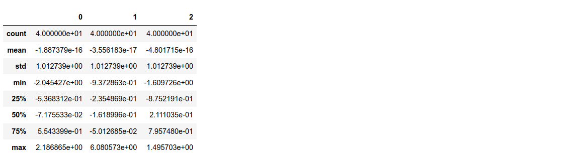
The DataFrame.describe() function allows us to check that both the train and test samples were successfully scaled:

1

df_train_scaled_sd.describe()

1

df_test_scaled_sd.describe()

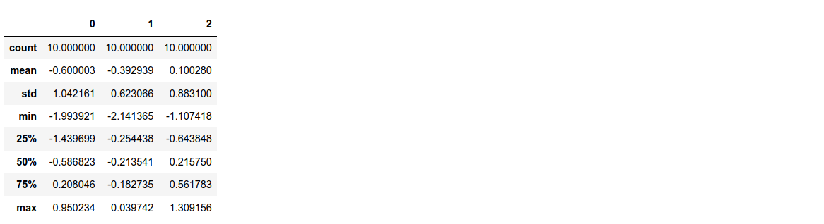
In the train sample, the mean and standard deviation are equal to 0 and 1 respectively, by definition of the standardizing transformation. But those quantities are relatively far from those values in the test sample. Of course, if the number of observations were much bigger, the difference would not be that notable (although this does not stand for the Cauchy distributed Y feature…).

PySpark

1
2
3
4
5
6
7
8
9

from pyspark.sql import SparkSession
# Specify the number of available cores in .master()
spark = SparkSession.builder.master('local[4]').appName('Scaling data with Spark').getOrCreate()

# Let us use the Pandas.DataFrame created above with NumPy/Pandas
df = spark.createDataFrame(df)

# Split the data into train/test samples
train, test = df.randomSplit([.8, .2], seed = 42)

As usual in Spark, we must first gather the features into one columns before applying any transformation.

1
2
3
4
5

# Gather the columns into one with a VectorAssembler, as usual in Spark
from pyspark.ml.feature import VectorAssembler
vector_assembler = VectorAssembler(inputCols=df.schema.names, outputCol="features")
train = vector_assembler.transform(train)
test = vector_assembler.transform(test)

This time only standardization will be done. As in scikit-learn, other scalers are available in Sparks’s MLlib: see here.

 1
 2
 3
 4
 5
 6
 7
 8
 9
10
11
12

# Standardize the data using only the train sample
# This is very similar to scikit-learn preprocessing workflow
from pyspark.ml.feature import StandardScaler
scaler = StandardScaler(
    inputCol="features",
    outputCol="scaledFeatures",
    withStd=True,
    withMean=True
)
scalerModel = scaler.fit(train)
train_scaled = scalerModel.transform(train)
test_scaled = scalerModel.transform(test)

The snippet below computes the specified summary statistics (mean and standard deviation in this case):

1
2
3
4

# Check the results are consistent
from pyspark.ml.stat import Summarizer
summarizer = Summarizer.metrics("mean", 'std')
train_scaled.select(summarizer.summary(train_scaled.scaledFeatures)).show(truncate=False)

R

Once again, the dataset is built as a tibble() using the random functions from Base R

 1
 2
 3
 4
 5
 6
 7
 8
 9
10
11
12
13
14
15
16

library(tidyverse)
library(caret)

set.seed(42)

# Build the dataset
df <- tibble(
  x = rnorm(50, mean = 2, sd = 2),
  y = rcauchy(50),
  z = runif(n = 50, min = 5, max = 10)
)

# Split into train/test samples
train_indexes <- sample(x = nrow(df), size = 0.8*nrow(df) )
df_train <- df %>% slice(train_indexes)
df_test <- df %>% slice(-train_indexes)

The easiest way: the caret package

We demonstrate both the standardization and the normalization. The scaling is basically done in three lines of code.

1
2
3
4
5
6
7

# Compute scaling parameters solely on the train sample
standardize_params <- preProcess(df_train, method = c("center", "scale"))
normalize_params <- preProcess(df_train, method = c("range"))

# For example, standardize both train and test samples
df_train_standardized_caret <- predict(standardize_params, df_train)
df_test_standardized_caret <- predict(standardize_params, df_test)

The old-school way: base R

There is not too much to say about it, this is quite straightforward if you know your way around the sweep() and apply() functions. Of course, the pipe %>% is not a base R feature but I use it for the sake of clarity.

1
2
3
4
5
6
7
8

# Compute scaling parameters solely on the train sample
means <- apply( X = df_train, MARGIN = 2, FUN = mean )
stdvs <- apply( X = df_train, MARGIN = 2, FUN = sd )

# Standardize the test sample
df_test_standardized_baseR <- df_test %>%
  sweep( MARGIN = 2, STATS = means, FUN = "-" ) %>%
  sweep( MARGIN = 2, STATS = stdvs, FUN = "/" )

the hardest way: Tidyverse’s dplyr

Also the best way in some cases. For instance, if only a subset of features have to be scaled. This can be achieved efficiently with the across() available in dplyr 1.0.0. For example, features whose name starts with a given string or numeric ones. More on across() here.

 1
 2
 3
 4
 5
 6
 7
 8
 9
10
11

# Compute scaling parameters solely on the train sample
means <- df_train %>% summarise(across(everything(), mean))
stdvs <- df_train %>% summarise(across(everything(), sd))

# Standardize the test sample
df_test_standardized_dplyr <- df_test %>%
  rowwise() %>%
  mutate(
    (across(everything())-means)/stdvs
    ) %>%
  ungroup()

1
2
3
4

## Check the results are consistent
df_test_standardized_caret %>% summarise_all(mean)
df_test_standardized_baseR %>% summarise_all(mean)  
df_test_standardized_dplyr %>% summarise_all(mean) 

The results are all the same :)

Conclusion

Train-test splitting and scaling are fundamental stages of data preprocessing. In particular, scaling is necessary with a number of ML algorithms. Despite being a rather easy task, it requires specific tools to be achieved properly. Today we have seen that Python & R provide very efficient packages to scale data the right way. All the code presented in this article is available on my GitHub.

References

[1] IOFFE, Sergey, SZEGEDY, Christian: Batch Normalization: Accelerating Deep Network Training by Reducing Internal Covariate Shift, Google Inc., 2015.

See also

• Full Stack Data Engineering
• A multi container ML app (1/3): Docker
• An asymmetric loss for regression models
• Interpretable machine learning with SHAP
• Image recognition with PyTorch and fastai