Run the Shiny CLT app at https://datatrigger.shinyapps.io/CLT_Visualization/
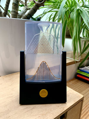
The Galton Board
As an introduction to this post, let me introduce one of the geekiest objects I own: a Galton Board, also known as a bean machine or a quincunx.
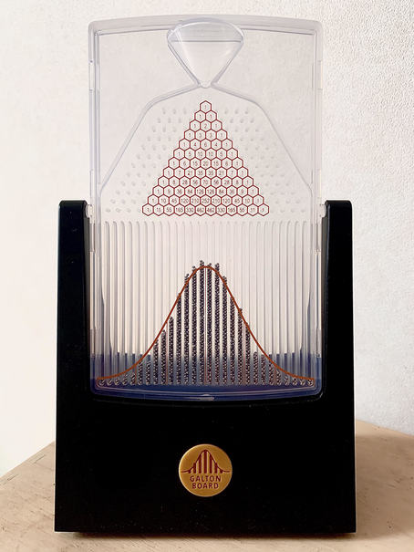
It is named after the polymath of genius Francis Galton, well-known for coming with the statistical term regression. I bought it after watching Vsauce’s video on the subject. It is a great illustration of the central limit theorem because it shows how a binomial distribution — as the sum of Bernoulli variables — approximates a normal distribution when the number of trials $n$ is large enough.
The central limit theorem
The CLT comes in many tastes and flavors and it can be found in about a zillion math books. However, writing this article without explicitly mentioning at least its “standard” version is inconceivable ! Let $(X_i)_{i \in \mathbb{N}}$ be a sequence of independent and identically distributed random variables. Suppose that the associated distribution admits finite expected value $\mu$ and variance $\sigma²$. Then the sequence:
converges in distribution to the standard normal distribution $\mathcal{N}(0,1)$, where
Visualizing the CLT
The Shiny CLT app is currently deployed on shinyapps.io. It computes samples, then the mean of these samples, for the following distributions:
- Continous distributions: Cauchy, exponential, log-normal and uniform
- Discrete distributions: binomial and Poisson
The Cauchy distribution does not satisfy the CLT hypotheses as its mean and variance are undefined, consequently to the divergence of the associated integrals. The density shown in the Shiny app has its location parameter $x_0$ set to 0 and its scale $\gamma$ set to 1. We can see how close it is to the density of a standard normal distribution, except for the heavier tails. The parameters of the other distributions are the default parameters of the random variate generation functions available in the R package stats.
For each of the studied distributions, the app displays a histogram of the computed means. It lets the user define the size $n$ of the samples generated to compute those means, as well as the number of samples. The number of bins for the histograms is also adjustable. It corresponds to the parameter bins in ggplot2’s geom_histogram().
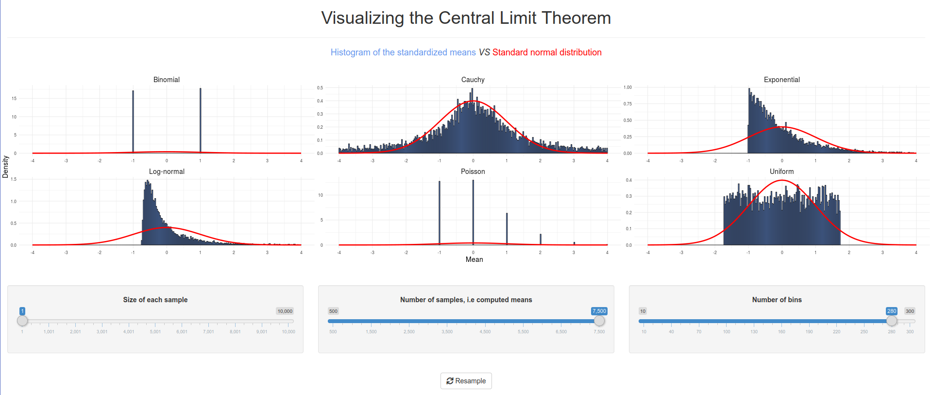
When the size of each sample is equal to 1, then the computed mean of a given sample is just the value of its unique observation. In this case, we obtain histograms of the standardized original distributions:
We can see that as we increase the sample size, the histograms of the means gets more and more close to the density of a standard normal distribution. That is the beauty of the central limit theorem shining live:
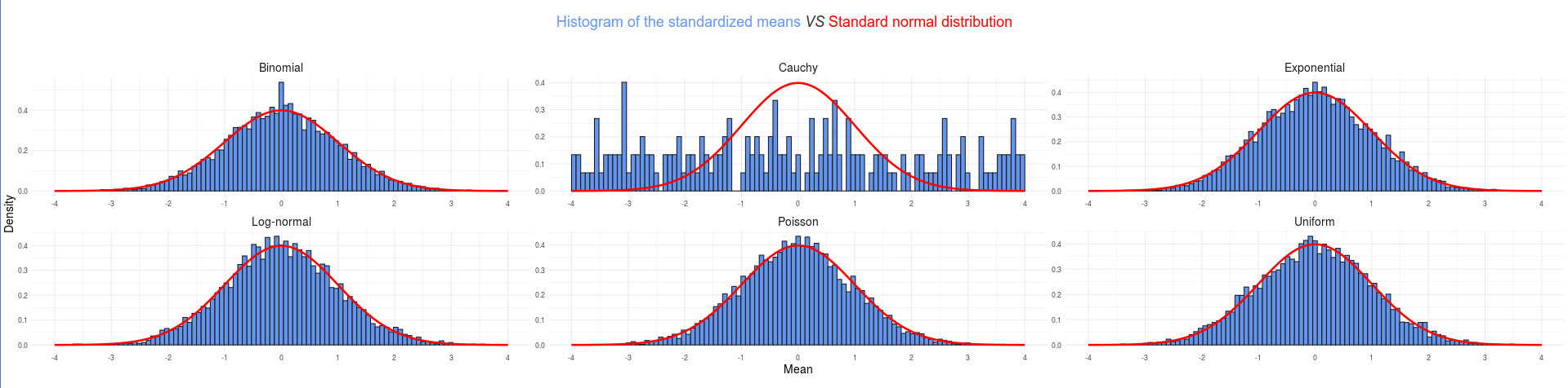
The Cauchy distribution magnificently stands out as a “counterexample” of the CLT. As usual, the source code of the Shiny app is available on GitHub.