Outlier detection

What is an outlier ?

An outlier can be defined as an observation that appears to deviate markedly from other members of the sample in which it occurs [1]. The question that immediately arises is the following: is this observation inconsistent ? Meaning was it generated by a different mechanism, or is it just “bad luck” ? This problem is kind of important, since as François Chollet (creator of the API Keras) recently tweeted:
 

All datasets have outliers. And your production data will always feature outliers of a kind never seen in your training data.

— François Chollet (@fchollet) August 21, 2020

Different ways to identify outliers

There are quite a few methods to study outliers and eventually detect anomalies. They can be classified in several ways. Some methods are global as opposed to local algorithms, which only use the $k \in \mathbb{N}$ nearest neighbors. Algorithms like DBSCAN [2] assign a binary label to observations (outlier or not) while others (Isolation Forest [3], Local Outlier Factor [4] or more recently Local Distance-based Outlier Factor [5]) output an anomaly score. Other criteria are to be considered depending on the use case: parametric or not, supervised or unsupervised, etc…

Local Outlier Factor

Today, we will focus mainly on a specific algorithm, namely Local Outlier Factor. In my opinions, this method is well adapted to real-world anomaly detection for several reasons. First, it is unsupervised, hence they do not require preliminary time-consuming - and possibly unreliable - work to characterize abnormal observations. Secondly, a list of individuals ranked by decreasing anomaly score can be generated with this methods. This is very a big advantage over binary algorithms because it allows the user to retain/inspect only a given number of observations, according to his time and need. Thirdly, Local Outlier Factor is distribution-free. This is crucial because estimating distribution can be very challenging, especially if the observations belong to a high-dimensional space (see the curse of dimensionality). Lastly, Local Outlier Factor is, well, local. This allows LOF to perform well in configurations like this one (code for this plot available in the R script):

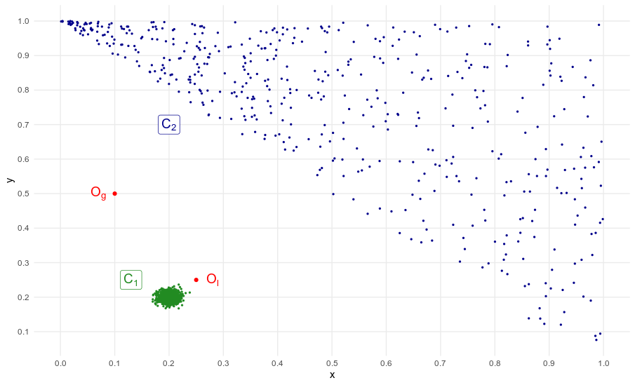
This dataset will be our case study.

So, why does it have to be local ?

In the example above, largely inspired from the original LOF paper [4], $C_1$/$C_2$ are cluster and $O_l$/$O_g$ are outliers. $O_l$ is considered a local outlier because the distance between $C_1$ and $O_l$ is not greater than say the average distance between $C_2$’s neighboring points. On the contrary, $O_g$ is clearly a global outlier. In this situation, a global anomaly detection method will most likely identify as outlier only $O_g$, or $O_g$, $O_l$ and a many observations from $C_2$. Only a local method will detect $O_g$ and $O_l$. This point is important because real-world data is often scattered, with several clusters of different densities.

The input parameter k

The LOF method is a k-nearest neighbors style algorithm [4], so it requires an integer $k$ as an input argument. Its creators were nice enough to give guidelines for choosing a set of appropriate values for the parameter $k$.
First, $k=10$ appears to be a reasonable lower bound. Indeed if $k < 10$, the authors have empirically observed that the standard deviation of LOF computed on observations from a 2D Gaussian sample is unstable, and that some observations from a 2D uniform distribution are clearly identified as outliers, which is problematic in this case. Alternatively, the lower bound for $k$ can be regarded as the minimal number of observations a set has to contain in order to be considered a cluster.
Secondly, the upper bound for k can be regarded as the highest number of outliers there can be relatively to a given cluster. In our case study, we only have two outliers so it is unnecessary to go well above 10. We decide to compute LOF for $10 \leq k \leq 15$. As the creators suggest, we will retain the maximum value i.e $\underset{10 \leq k \leq 15}{max} \ LOF_k(observation)$ for each observation.

Interpretation of the Local Outlier Factor

Let $C$ be a set of observations and $k$ the input parameter presented above. Then for all $p \in C$ such that the k-nearest neighbors of $p$ and their k-nearest neighbors also belong to $C$, the following inequality stands [4]: $$\frac{1}{1+\epsilon} \leq \ LOF_{Minpts}(p) \ \leq 1+\epsilon$$ where $\epsilon$ is a measure of $C$’s “looseness”. Hence if $C$ is a “tight” cluster, then the local outlier factor of all the observations that belong to $C$ is close to 1. On the contrary, the LOF of an outlier is well above 1.

LOF vs Isolation Forest: let the battle begin

Now, let us see how LOF performs on the dataset plotted above, and compare the results with the global method Isolation Forest. The results presented below were generated by the R script. The Python script gives very similar results, with fluctuations due to random number generation.

Dataset

First, let us generate the data. We use a normal distribution for $C_1$ and a uniform distribution for $C_2$, then we manually add the two outliers to the dataset. We also add an id column as a primary key for the observations.

Python

 1
 2
 3
 4
 5
 6
 7
 8
 9
10
11
12
13
14
15
16
17
18
19
20
21
22
23
24
25
26
27
28
29
30

import pandas as pd
from numpy.random import *

# Generate data
seed(1)

disk = pd.DataFrame({
    'x': normal(0.2, 0.01, 1000),
    'y': normal(0.2, 0.01, 1000),
    'category': 'Disk'
})

# This is why I like dplyr and mutate():
x_values = uniform(0, 1, 500)
y_values = list(map(lambda x: float(uniform(1-x, 1, 1)), x_values))

triangle = pd.DataFrame({
    'x': x_values,
    'y': y_values,
    'category': 'Triangle'
})

outliers = pd.DataFrame({
    'x': [0.25, 0.1],
    'y': [0.25, 0.5],
    'category': ['Local outlier', 'Global outlier']
})

df = pd.concat([disk, triangle, outliers], axis=0).reset_index(drop=True)
ax1 = df.plot.scatter(x = 'x', y = 'y')

R

 1
 2
 3
 4
 5
 6
 7
 8
 9
10
11
12
13
14
15
16
17
18
19
20
21
22
23
24
25
26
27
28
29
30
31
32

# Generate data
set.seed(1)

disk <- tibble(
  x = rnorm(1000, 0.2, 0.01),
  y = rnorm(1000, 0.2, 0.01),
  category = 'Disk'
)

triangle <- tibble(
  x = runif(500, 0, 1),
  y = runif(500, 1-x, 1),
  category = 'Triangle'
)

outliers <- tribble(
  ~x, ~y, ~category,
  0.25, 0.25, 'Local outlier',
  0.1, 0.5, 'Global outlier'
)

df <- disk %>%
  bind_rows(
    triangle
  ) %>%
  bind_rows(
    outliers
  ) %>%
  mutate(
    id = row_number()
  ) %>%
  select(id, everything())

We get the dataset we already showed above, with two clusters, one global outlier and one local outlier.

LOF

Now let us begin the outlier detection process. As explained before, we compute the LOF of each observation for $10 \leq k \leq 15$, then we retain the maximal value.

Python

We use the beloved module scikit-learn.

 1
 2
 3
 4
 5
 6
 7
 8
 9
10

# Local Outlier Factor
from sklearn.neighbors import LocalOutlierFactor

for k in range(10, 16):
    lof = LocalOutlierFactor(n_neighbors = k)
    df['lof_' + str(k)] = lof.fit(df[['x', 'y']]).negative_outlier_factor_

# Computation of the maximal LOF of each observation
df_results = df.melt(id_vars=['x', 'y', 'category'], var_name='k', value_name = 'lof').drop(columns = 'k').groupby(['x', 'y', 'category']).min()
df_results = df_results.sort_values(by = 'lof').reset_index()

R

We use the R package Rlof and the function rlof().

 1
 2
 3
 4
 5
 6
 7
 8
 9
10
11
12
13
14
15
16
17
18
19
20
21
22
23
24
25
26
27
28
29
30
31
32
33
34

# Local Outlier Factor
df_lof <- df
# let us use 4 cores
cluster <- makePSOCKcluster(4)
registerDoParallel(cluster)

for(i in seq(10,15)){
  df_lof <- df_lof %>%
    bind_cols(
      tibble( !!str_c('k = ', i) := Rlof::lof(data = df %>% select(x, y), k = i) )
    )
}

stopCluster(cluster)
  
# Computation of the maximal LOF of each observation
df_lof_agg <- df_lof %>%
  pivot_longer(
    cols = starts_with('k'),
    names_to = 'k',
    values_to = 'lof'
  ) %>%
  group_by(id) %>%
  summarise(
    lof_max = max(lof)
  )

# Results
df_lof <- df_lof %>%
  inner_join(
    df_lof_agg,
    by = 'id'
  ) %>%
  arrange(desc(lof_max))

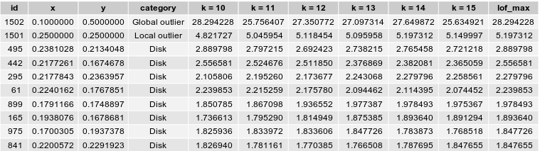
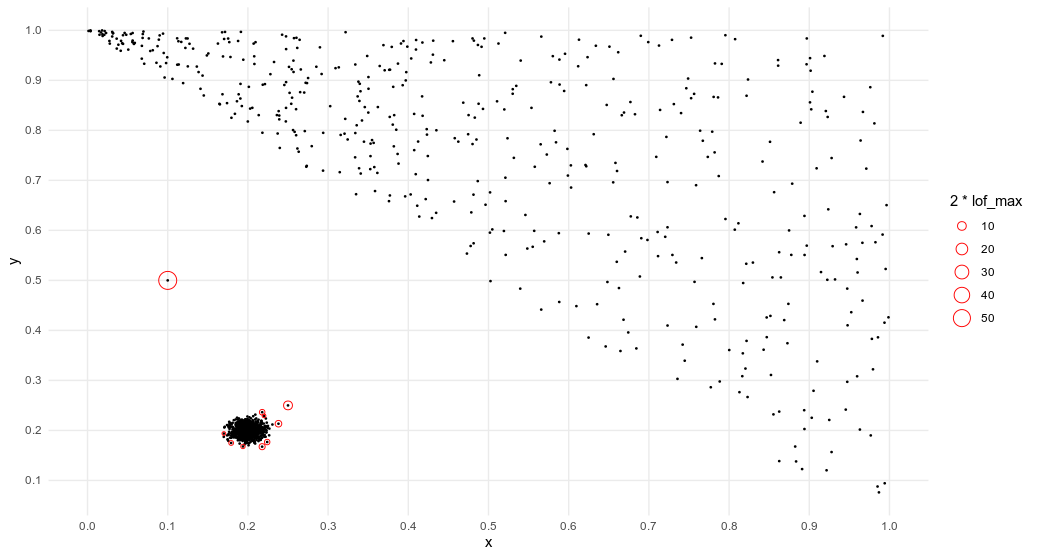
Success ! The Local Outlier Factor algorithm clearly identifies the two outliers of our datasets, as the anomaly score of the these points are the highest and well above 1. Below is a representation of the 10 observations with the highest LOF. They are circled with a radius proportional to their score.

Comparison with Isolation Forest

Python

1
2
3
4
5
6

# Isolation forest
from sklearn.ensemble import IsolationForest

isolation_forest = IsolationForest(n_estimators = 500, max_samples = df.shape[0], random_state = 1)
df_results['if'] = isolation_forest.fit(df_results[['x', 'y']]).score_samples(df_results[['x', 'y']])
df_results.sort_values(by = 'if')

R

We use the R package solitude.

 1
 2
 3
 4
 5
 6
 7
 8
 9
10
11
12
13
14
15
16
17
18

# Isolation forest
# Creation of an Isolation Forest with default parameters
isolation_forest<- isolationForest$new(
  sample_size = nrow(df),
  num_trees = 500,
  replace = FALSE,
  seed = 1,
  nproc = 4
)
# Fit to the data
isolation_forest$fit(df %>% select(x, y) %>% as.data.frame())

# Compute anomaly scores and append them to the original data
df_if <- df %>%
  mutate(
    if_anomaly_score = isolation_forest$predict(df %>% select(x, y) %>% as.data.frame()) %>% pull(anomaly_score)
  ) %>%
  arrange(desc(if_anomaly_score))

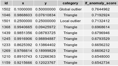
As a global anomaly detection, Isolation Forest clearly detects the outlier $O_g$. The anomaly score of this global outlier is the highest, and well above the second highest value. However, the Isolation Forest algorithm fails to distinctely identify the local outlier $O_l$. Even though its anomaly score is the third highest value of the dataset, it does not clearly stands out from the other anomaly scores.

Conclusion

In my experience, Local Outlier Factor is one of the best methods to identify outliers and detect anomalies. We have seen that it works very well on today’s case study, but it is efficient in many other configurations. Nonetheless, LOF is admittedly one of the anomaly detection algorithms that requires the most computing power, particularly when applied on big datasets. Other than that, the fact that it is unsupervised, distribution-free, local (so well-adapted to multiple clusters of different densities) and that it outputs a real number are the reasons why it is the way to go.

All the code can be found on my Github.

References

[1] BARNETT, V., LEWIS, T., Outliers in Statistical Data, 1994. 3rd edition, John Wiley & Sons.
 
[2] ESTER, Martin, KRIEGEL, Hans-Peter, SANDER, Jiirg, XU, Xiaowei: A Density-Based Algorithm for Discovering Clusters in Large Spatial Databases with Noise. Institute for Computer Science, University of Munich, 1996.
 
[3] LIU, Fei Tony, TING, Kai Ming and ZHOU, Zhi-Hua: Isolation forest. Data Mining, 2008. ICDM 2008. Eighth IEEE International Conference on Data Mining.
 
[4] Markus M. Breunig, Hans-Peter Kriegel, Raymond T. Ng, Jörg Sander, *LOF: Identifying Density-Based Local Outliers
 
[5] ZHANG, K., HUTTER, M., JIN, H., New Local Distance-Based Outlier Detection Approach for Scattered Real-World Data, 2009.

See also

• Full Stack Data Engineering
• A multi container ML app (1/3): Docker
• An asymmetric loss for regression models
• Interpretable machine learning with SHAP
• Image recognition with PyTorch and fastai