Weighted Random Forest with Spark 3

Spark 3

The main new enhancement in PySpark 3 is the redesign of Pandas user-defined functions with Python type hints. Here we focus on another improvement that went a little bit more unnoticed, that is sample weights support added for a number of classifiers. Let us give random forest a try.

Load the credit card fraud dataset in a Spark Session

We work on the notoriously imbalanced credit card fraud detection dataset available on Kaggle. Let us instantiate a SparkSession and load the data into it. I use the four cores available on my machine using the option master('local[4]').

1
2
3
4
5
6
7
8

# Initialize a Spark Session
from pyspark.sql import SparkSession
# Specify the number of available cores in .master()
spark = SparkSession.builder.master('local[4]').appName('Weighted Random Forest with Spark 3').getOrCreate()

# Get the data here: https://www.kaggle.com/mlg-ulb/creditcardfraud
csv_file = ".../creditcard.csv"
df = spark.read.format("csv").option("inferSchema", "true").option("header", "true").load(csv_file)

1

print(df)

The ‘Time’ column is to be deleted since it contains the seconds elapsed between each transaction and the first transaction. This is irrelevant in my opinion. We also rename some columns for our good taste.

1

df = df.drop('Time').withColumnRenamed('Amount', 'amount').withColumnRenamed('Class', 'outcome')

Count the frauds and weight them

1
2
3
4

# Check imbalance and compute weights
import pandas as pd
counts = df.groupBy('outcome').count().toPandas()
print(counts)

We only have 492 frauds out of 284807 transactions. A rather imbalanced dataset indeed. This is the reason why we compute a weight for each observation, according to its class (i.e fraud / not fraud). We will use the following popular method, even though there seems to be no strong consensus at the moment among the ML community regarding this subject: $$w_i := \frac{n}{n_i * C}$$

Where $C$ is the number of classes (today, $C = 2$), $i \in {1…C}$, $n$ is the total number of observations and $n_i$ the number of observations of class $i$.

 1
 2
 3
 4
 5
 6
 7
 8
 9
10
11
12
13
14
15
16
17

# Counts
count_fraud = counts[counts['outcome']==1]['count'].values[0]
count_total = counts['count'].sum()

# Weights
c = 2
weight_fraud = count_total / (c * count_fraud)
weight_no_fraud = count_total / (c * (count_total - count_fraud))

# Append weights to the dataset
from pyspark.sql.functions import col
from pyspark.sql.functions import when

df = df.withColumn("weight", when(col("outcome") ==1, weight_fraud).otherwise(weight_no_fraud))

# Check everything seems ok
df.select('outcome', 'weight').where(col('outcome')==1).show(3)

1

df.select('outcome', 'weight').where(col('outcome')==0).show(3)

We can also have a quick look at the features using the extremely useful describe() function. Since the result is agreggated data, it is no problem to convert it to a Pandas DataFrame in order to benefit from the much nicer displaying features of this library:

1

df.describe().toPandas()

All the features, except from ‘Amount’ come from a PCA on the original dataset, to keep it anonymous. Hence they are all centered in 0. No scaling is necessary to perform the random forest algorithm or the logistic regression.

Split the dataset and format data

1
2
3

# Split the dataset into train and test subsets
train, test = df.randomSplit([.8, .2], seed = 0)
print(f"""There are {train.count()} rows in the train set, and {test.count()} in the test set""")

There are 227805 rows in the train set, and 57002 in the test set.

1

test.where(col('outcome')==1).count()

101 frauds out of 492 ended up in the test set.

In Spark, all the dependent variable have to be nested in a column often named ‘features’. I think this way of pre-processing the data is an excellent idea because it avoids mistakes like forgetting columns or applying unintentional changes.

1
2
3
4
5

# Format the data for MLlib models
from pyspark.ml.feature import VectorAssembler
vector_assembler = VectorAssembler(inputCols=df.schema.names[:-2], outputCol="features")
train = vector_assembler.transform(train)
test = vector_assembler.transform(test)

Learning time, machine

Hyperparameter tuning is not the topic of this post, so We train four models with default parameters (except for numTrees because the default value - 20 - feels a bit low):

• rf: Random Forest
• rfw: Weighted Random Forest
• lr: Logistic Regression
• lrw: Weighted Logistic Regression

Hyperparameter tuning is not on the agenda, but we will certainly have a chance to do grid search and cross validation with PySpark on another day.

1
2
3
4
5

from pyspark.ml.classification import RandomForestClassifier

# Random Forest without weights
rf = RandomForestClassifier(numTrees = 200, featuresCol='features', labelCol='outcome', seed=0)
rf = rf.fit(train)

1
2
3

# Random Forest with weights
rfw = RandomForestClassifier(numTrees = 200, featuresCol='features', labelCol='outcome', weightCol='weight', seed=0)
rfw = rfw.fit(train)

1
2
3
4

# Logistic Regression without weights
from pyspark.ml.classification import LogisticRegression
lr = LogisticRegression(featuresCol='features', labelCol='outcome')
lr = lr.fit(train)

1
2
3

# Logistic Regression with weights
lrw = LogisticRegression(featuresCol='features', labelCol='outcome', weightCol='weight')
lrw = lrw.fit(train)

Predict the outcome and compute confusion matrices

We use the transform function to generate predictions.

1
2
3
4
5

# Predict the outcome for the test set using the four different models computed above
res_rf = rf.transform(test)
res_rfw = rfw.transform(test)
res_lr = lr.transform(test)
res_lrw = lrw.transform(test)

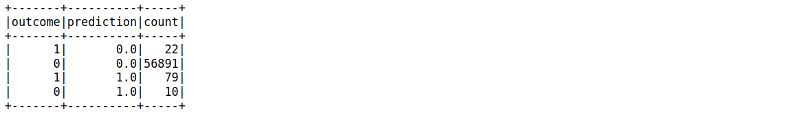
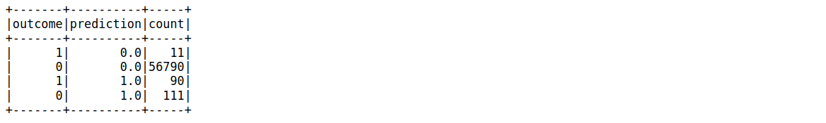
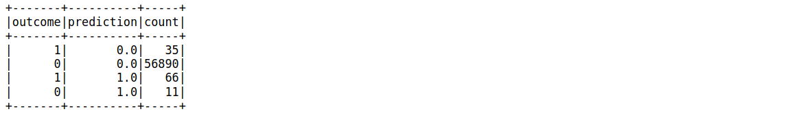
Now let us have a look at the confusion matrices for the test set:

1
2
3
4

# Let us have a look at the confusion matrices on the test set

# Random Forest without weights
res_rf.groupBy('outcome', 'prediction').count().show()

1
2

# Random Forest with weights
res_rfw.groupBy('outcome', 'prediction').count().show()

1
2

# Logistic Regression without weights
res_lr.groupBy('outcome', 'prediction').count().show()

1
2

# Logistic Regression with weights
res_lrw.groupBy('outcome', 'prediction').count().show()

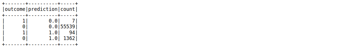
From bottom to top, we can see that the logistic regression without weights performs very well when it comes to detecting actual fraud. However, this comes at the cost of wrongly identifying a lot of wholesome transactions as frauds. The opposite disequilibrium happens with the standard logistic regression, with only roughly $\frac{2}{3}$ of frauds legitimately detected. However, only 11 out of 56 901 wholesome transactions are identified as fraud, which is surprisingly low. Of course, the same experiment with different train/test splits should be conducted before jumping to conclusions.

As for random forests, the weighted model shows almost the same performance as the weighted logistic regression regarding real frauds: 90 correct guesses instead of 94. But this time, the number of wholesome transactions mistakenly identified as frauds is divided by ten. This kind of model should be considered when the cost of false positive is relatively low compared to the cost of false negative. What about plain old unweighted random forest model ? It identifies wholesome transactions extremely well, like the basic logistic regression (10 out of 56 901). However, the model is able to rise the precision (as in precision vs recall) to approximately $\frac{4}{5}$. Put another way, the precision was increased by around 15% with random forest instead of logistic regression.

We will not dive into the hot topic of evaluation metrics for imbalanced classification. However, we give an example below with the computation of the area under the Precision-Recall curve:

1
2
3
4
5

# Compute the area under the PR curve
from pyspark.ml.evaluation import BinaryClassificationEvaluator

pr = BinaryClassificationEvaluator(rawPredictionCol = 'prediction', labelCol="outcome", metricName="areaUnderPR")
pr.evaluate(res_rf)

Conclusion

Weighted or not, random forest performs well at detecting fraud in comparison with logistic regression. However, having the option of weighting observations is an extremely useful feature as it allows the user to lean the model’s performance toward a specific phenomenon. In fraud detection for example, a weighted model is a valid choice if the cost of fraud is high regarding the cost of mistakenly identifying wholesome events as frauds.

You can find the full notebook in this GitHub repository.

See also

• Full Stack Data Engineering
• A multi container ML app (1/3): Docker
• An asymmetric loss for regression models
• Interpretable machine learning with SHAP
• Image recognition with PyTorch and fastai