Full notebook available on GitHub
In the context of regression, there are a few real-world situations in which users would rather get positive errors than negative ones (or the opposite), while still wanting estimations as accurate as possible:
- Forecasting supply needs for materials critical for production: you’d better have too much than be short
- Time to delivery: clients may be much more bothered by delay than by earlier-than-expected events
- Estimating insurance premium: companies may overestimate costs rather than underestimate them to remain profitable
Let’s implement a custom asymmetric loss for this purpose. We will use this Kaggle dataset about used motorcycles’ prices. We will drive the regression model towards underpredicting values using the linear-exponential loss. This way, the bikes would generally be sold at a higher price than expected, while keeping accurate estimations on average. This approach is interesting from a seller’s perspective as it tends to avoid bad surprises.
An asymmetric cost function for regression: the linear-exponential loss
Surprisingly, I have found very little data about asymmetric loss functions in the context of regression. Most of the papers/threads I have came across mention variations of the standard quadratic loss (see here and there) or other impractical functions. Why impractical? Because these losses do not have “smooth” derivatives! This is unfortunate for us Machine Learning practioners, who abide by the almighty gradient descent approach.
This paper [1] and a few Stack Overflow / Cross Validated threads bring up the linear-exponential loss, sometime called LINEX. Let us denote it by ($lexp$). It is defined as follows:
$$lexp \colon E \longmapsto b \cdot [e^{a \cdot E} - a \cdot E - 1]$$
where $E$ is the difference between the observed value and the predicted value, i.e $E:=y-\hat{y}$.
When $a$ is close to 0, then $lexp(E) \sim b \cdot \frac{a^2 \cdot E^2}{2} + o(E^2)$ (see Taylor series of $exp$). So, let us set $b=\frac{2}{a^2}$. This way, we will have $lexp(E) \approx E^2$ when $a$ is small. When $a$ increases, the “asymmetry” of the loss increases as well:
As this function is infinitely differentiable, it can very well be implemented as a custom loss in popular Machine Learning libraries: see with PyTorch or Keras for example.
Let us give an XGBoost example. To train such a model with this custom loss, we will need to provide its first and second order derivatives with respect to the prediction $\hat{y}$ (see section 2.2 of the XGBoost paper, or the example in the doc):
$$ \begin{cases} lexp (y, \hat{y}) = \frac{2}{a^2} \cdot [e^{a \cdot (\hat{y}-y)} - a \cdot (\hat{y}-y) - 1] \\[6pt] \frac{\partial lexp}{\partial \hat{y}}(y, \hat{y}) = \frac{2}{a} \cdot [e^{a \cdot (\hat{y}-y)} - 1] \\[6pt] \frac{\partial^{2} lexp}{\partial {\hat{y}}^2}(y, \hat{y}) = 2 \cdot e^{a \cdot (\hat{y}-y)} \end{cases} $$
Here we have defined the error as the unconventional $\hat{y}-y$. The point is to avoid minus signs all over the place when computing derivatives. This will lead to penalize overestimations more than underestimation: overall, the model will underestimate. If we want to train the regressor the other way around, then we will swap $\hat{y}-y$ for the “usual” $y-\hat{y}$, keeping in mind the following high school classics:
$$ \begin{cases} \frac{\partial}{\partial x}f(\text{-} x) = \text{-} f’(\text{-} x) \\[6pt] \frac{\partial^2}{\partial x^2}f(\text{-} x) = f’’(\text{-} x) \end{cases} $$
Technical note: using 128-bit floats is advised when implementing this loss. Else overflow errors may arise because of skyrocketing values in the exponential.
Results
Let us compare the usual squared error and the linear-exponential loss using a few metrics: RMSE, mean, median and 95th percentile of the residuals on the test set. These numbers are very dependent on the train-test split because the dataset is very small. In order to get stable values, we use the following method:
- For each $a$ value:
- Make a random train-test split
- Build a squared-error-loss model and a linear-exponential-loss model, retrieve residuals
- Repeat 500 times
- Compute aggregated metrics over the entire collection of residuals
Note: we did not perform hyperparameter tuning as accuracy is not the purpose of this experiment. Default values are used for both the losses.
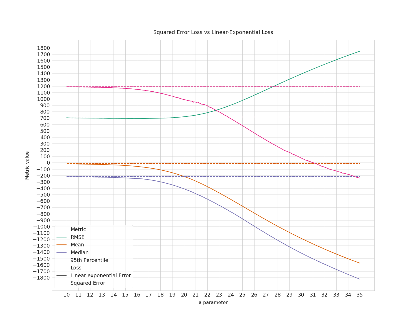
There is an interesting phenomenon happening between $a \approx 13$ and $a \approx 20$: the mean/median/perc. 95 start decreasing but the overall RMSE does not degrade. In other words, we are actually achieving underestimation without degrading the accuracy of the model.
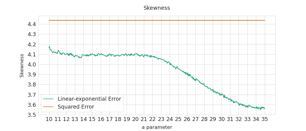
When $a=20$, the RMSE is the same for the two losses but the prices are estimated 200 dollars lower, on average. This means the linear-exponential loss allows the errors distribution to be skewed. Actually, in this case the squared-error-loss residuals are initially skewed to the right, as shown below. The linear-exponential loss “unskews” the residuals to the left.
An overcomplicated solution?
Recall that the point of all this is to drive the model towards underestimation, without loosing accuracy if possible. The linear-exponential loss is asymmetric (–> underestimation) but still aims at achieving 0 error (–> accuracy). These two characteristics appear to make this loss successful in that matter.
What if, instead of implementing this complicated custom loss, we just lowered the predictions by a fixed quantity? On the basis that the squared-loss errors average to 0 on the test set, we could just subtract 100 dollars to every prediction to achieve on overall underprediction of 100 dollars, on average. Now, we are doing underestimation without aiming at the actual price, but aiming at a minus-100-dollar error, on average. That is why I call such a loss a decentered squared error loss.
Below are the RMSEs of both losses (linear-exponential/decentered squared) when they achieve the same mean error. For instance, when both losses are adjusted to yield a 100 dollars average underestimation on the test set, the linear-exponential loss’ RMSE is about 695 dollars, whereas the decentered loss’ RMSE is about 721 dollars.
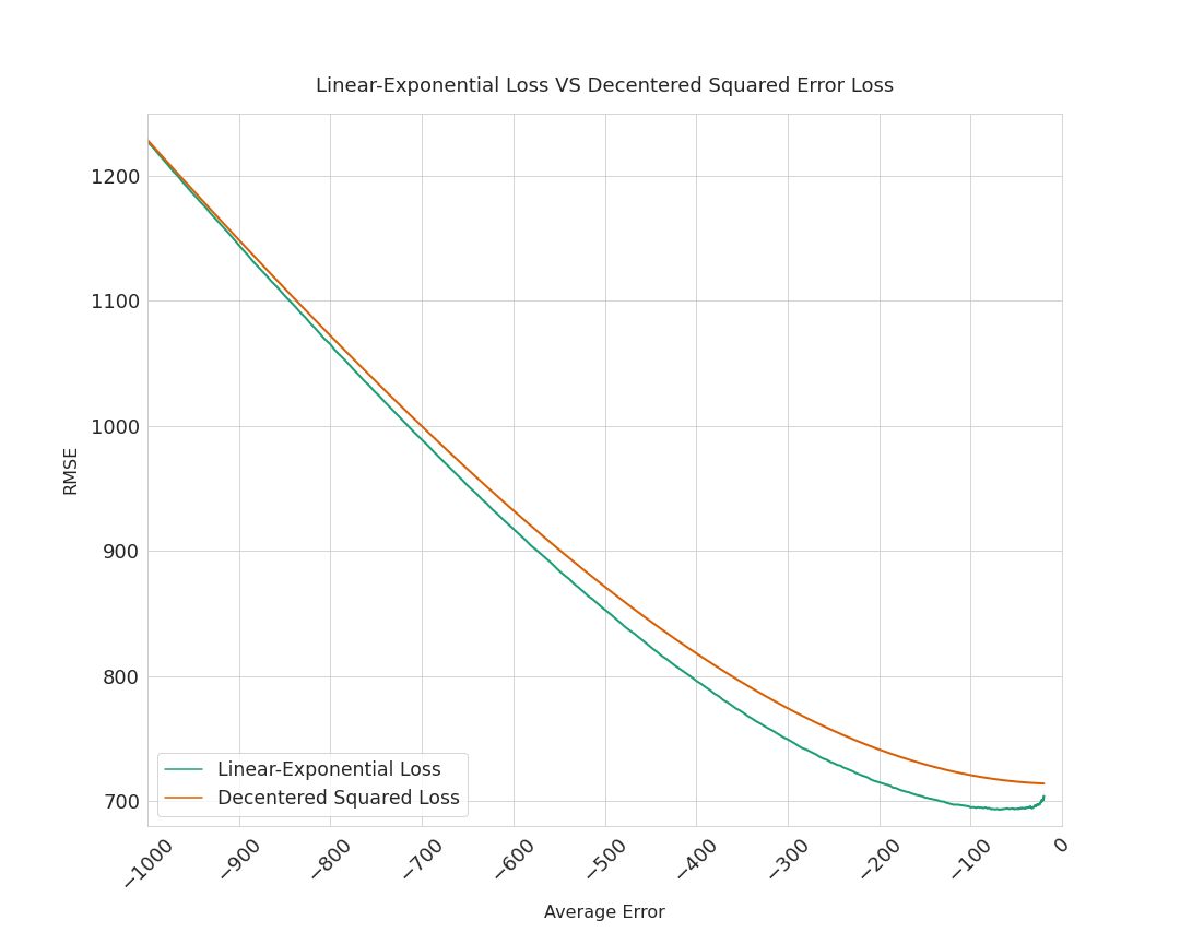
Although it is difficult to determine if the gap observed below is significant or not without further analysis (other datasets, other hyperparameter tunings…), this piece of information seems to be in favor of the linear-exponential loss’ relevance. An additional remark: when the average test error starts decreasing (read the plot from right to left), the decentered loss’ RMSE increases straight away, whereas the linex loss’ RMSE decreases first, before rising up again. So, with the linex loss, there is an interesting tradeoff between underestimation and accuracy.
Conclusion
Coming back to our used motorcycles prices. When a=19.65, the RMSE is the same wether the model is trained with the usual squared error loss or with the linear-exponential loss. However, the predictions are lowered by 180 dollars, on average. See the distributions of the residuals below:
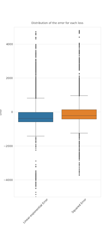
So, we have been able to drive our model towards underestimation, without sacrificing accuracy. Even more underestimation could be achieved by increasing the parameter a, but this would also increase RMSE.
References
[1] N. Khatun, M. A. Matin. A Study on LINEX Loss Function with Different Estimating Methods. Department of Statistics, Jahangirnagar University, Savar, Dhaka, Bangladesh, 2020.