Gradient tree boosting in the cloud

Introduction

The topic of the present post originates from the superconductivity dataset — available on the UCI Machine Learning Repository — and the associated paper [1]. The problem consists in predicting the critical temperature $T_c$ of superconductors. At or below this temperature, such a compound conducts current with zero resistance, hence eliminating power loss due to Joule heating. Surprisingly enough, the scientific community has failed to model $T_c$ since the discovery of superconductivity by Dutch physicist Heike Kamerlingh Onnes in 1911.

In his study [1], Kam Hamidieh builds a gradient boosted trees using the XGBoost algorithm. He ends up with an out-of-sample RMSE of 9.5 °K. Let us see how the LightGBM framework performs on this specific task.

Data

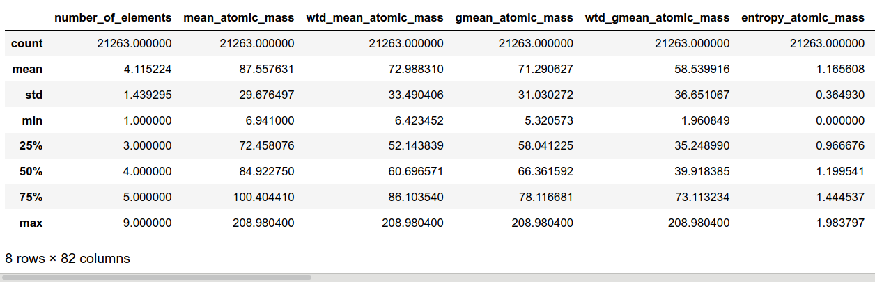
The dataset contains 21 263 superconductors described by 81 explanatory variables, and one more response variable $Tc$. We are cosily ensconced in the supervised learning framework, and more specifically, regression. The explanatory variables are all continuous and positive. They are related to the eight following physical properties of every atom forming the superconductor: atomic mass, first ionization energy, atomic radius, density, electron affinity, fusion heat, thermal conductivity and valence. For each of these characteristics, ten summary statistics are computed mean, weighted mean, geometric mean, entropy, range, etc… These quantities are the actual values of the independent variables. As a consequence, we get 8*10 = 80 highly correlated features. In this context, leaning towards tree-based ensemble methods seems reasonable. The eighty-first input variable is the number of atoms in the superconductor molecule.

1
2
3

import pandas
df = pd.read_csv("train.csv")
df.describe()

More information on data preparation, feature extraction as well as a descriptive analysis of the dataset are available in the original paper [1]. The following block attests that there are no missing values

1

print(f'There are {df.isna().sum().sum()} missing values in the dataset.')

XGBoost & LightGBM

XGBoost [2] and LightGBM [3] are slightly different implementations of gradient boosted trees. LightGBM is often considered as one as the fastest, most accurate and most efficient algorithm. The authors of the LightGBM documentation stress this point to a great extent. Although this may be correct in given situations, this Kaggle discussion shows that it depends on various parameters including the number of features, memory limitations, convergence and GPU vs CPU.

Let us see what happens with the superconductivity dataset. We will use the native Python API in both case to stay as objective as possible. Nonetheless, there are scikit-learn wrappers for both libraries. They are particularly useful with their integration to the sklearn.grid_search module.

Hardware

As my personal machine is getting quite old, the following computations were carried out in the cloud. We used a P4000 instance on Paperspace Gradient. We only used the CPU, although it is possible to use GPU both with LightGBM and XGBoost.

First test

In this part, we train a LightGBM model using the parameters provided by Kam Hamidieh in his paper. They were found with a grid search with cross-validation. We had to make a heavy use of LightGBM documentation to do an appropriate translation of these XGBoost parameters. To make an honest comparison with the original work, we use the same method to estimate the out-of-sample RMSE, that is:

• Split the data into random train and test subsets with 2/3 of the rows for training.
• Fit the model using the train data and compute the RMSE on the test sample.
• Repeat 25 times and retain the average RSME on the test data.

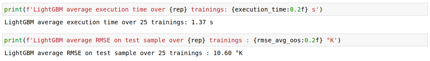
LightGBM

 1
 2
 3
 4
 5
 6
 7
 8
 9
10
11
12
13
14
15
16
17
18
19
20
21
22
23
24
25
26
27
28
29
30
31
32
33
34
35
36
37
38
39
40
41
42
43

# LightGBM parameters based on the original paper https://arxiv.org/abs/1803.10260
parameters_lgbm = {
    'boosting_type': 'gbdt',
    'objective': 'regression',
    'metric': 'l2',
    'learning_rate': 0.02,
    'max_depth' 16,
    'min_data_in_leaf' 1,
    'feature_fraction': 0.5,
    'bagging_fraction': 0.5,
    'bagging_freq': 1
}
num_trees = 374

# Train 25 models with the same parameters on 25 different train-test split samples
# and compute average RMSE on test samples
rep = 25
rmse = []
execution_time = []

seed(42)
for i in range(rep):
    # Format data for LightGBM
    train, test = train_test_split(df, test_size = 1/3)
    train_lgbm = lgb.Dataset(train[train.columns[:-1]], label=train[train.columns[-1:]])
    test_x = test[test.columns[:-1]]
    test_y = test[test.columns[-1:]]
    start = time()
    # Training
    lgbm = lgb.train(
        params = parameters_lgbm,
        train_set = train_lgbm,
        num_boost_round = num_trees
        )
    training_time = time() - start
    # Out of train sample predictions and metrics
    pred_y = lgbm.predict(test_x)
    rmse.append(mean_squared_error(test_y, pred_y) ** 0.5)
    execution_time.append(training_time)

# Compute average RMSE / Computing time
rmse_avg_oos = sum(rmse)/len(rmse)
execution_time = sum(execution_time)/len(execution_time)

XGBoost

 1
 2
 3
 4
 5
 6
 7
 8
 9
10
11
12
13
14
15
16
17
18
19
20
21
22
23
24
25
26
27
28
29
30
31
32
33
34
35
36

# XGBoost parameters based on the original paper https://arxiv.org/abs/1803.10260
parameters_xgb = {
    'booster': 'gbtree',
    'objective': 'reg:squarederror',
    'eta': 0.02,
    'max_depth' 16,
    'min_child_weight' 1,
    'colsample_bytree': 0.5,
    'subsample': 0.5
}
rmse = []
execution_time = []

seed(42)
for i in range(rep):
    # Format data for XGBoost
    train, test = train_test_split(df, test_size = 1/3)
    test_y = test[test.columns[-1:]]
    train_xgb = xgb.DMatrix(train[train.columns[:-1]], label=train[train.columns[-1:]])
    test_xgb = xgb.DMatrix(test[test.columns[:-1]], label = test_y)
    start = time()
    # Training
    xgbm = xgb.train(
        params = parameters_xgb,
        dtrain = train_xgb,
        num_boost_round = num_trees
        )
    training_time = time() - start
    # Out of train sample predictions and metrics
    pred_y = xgbm.predict(test_xgb)
    rmse.append(mean_squared_error(test_y, pred_y) ** 0.5)
    execution_time.append(training_time)

# Compute average RMSE / Computing time
rmse_avg_oos = sum(rmse)/len(rmse)
execution_time = sum(execution_time)/len(execution_time)

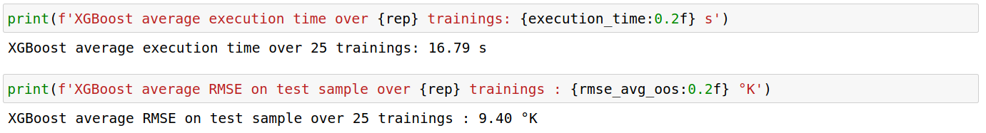
Using the same set of parameters in both libraries, LightGBM was approximately 12 times faster than XGBoost. However, the out-of-sample RMSE is 1.20 °K off in comparison with XGBoost’s performance.

A home-made grid search for appropriate LightGBM parameters

Let us try to improve the LightGBM model. Could we get lower RMSE and execution time than with XGBoost ? In this part, we do not dive into a meticulous grid search, but we implement an attempt based on the following recommendations from the LightGBM documentation to increase accuracy:

• Use large max_bin (may be slower)
• Use small learning_rate with large num_iterations
• Use large num_leaves (may cause over-fitting)

For each combination of all the other parameters, the number of iterations/trees i.e num_boost_round is selected through 5-fold cross-validation. In the end, we select the set of parameters that does best on the test sample.

 1
 2
 3
 4
 5
 6
 7
 8
 9
10
11
12
13
14
15
16
17
18
19
20
21
22
23
24
25
26
27
28
29
30
31
32
33
34
35
36
37
38
39
40
41
42
43
44
45
46
47
48
49
50
51
52
53
54
55
56
57
58
59
60
61
62
63
64
65
66
67
68
69

# Number of iterations
num_trees = 2000
early_stop = 10

# Parameters to be "grid searched"
eta_list = [0.02, 0.005, 0.001]
num_leaves_list = [100, 500, 1000]
max_bin_list = [255, 511, 1023]
min_data_in_leaf_list = [1, 20]

# Data
seed(42)
train, test = train_test_split(df, test_size = 1/3)
# free_raw_data must be set to False because it is reused
# when building the train data with a different max_bin parameter
train_lgbm = lgb.Dataset(train[train.columns[:-1]], label=train[train.columns[-1:]], free_raw_data = False)
test_x = test[test.columns[:-1]]
test_y = test[test.columns[-1:]]

parameters_lgbm_list = []
rmse_list = []

# Grid search
for eta in eta_list:
    for num_leaves in num_leaves_list:
        for max_bin in max_bin_list:
            for min_data_in_leaf in min_data_in_leaf_list:
            
                parameters_lgbm = {
                    'boosting_type': 'gbdt',
                    'objective': 'regression',
                    'metric': 'l2',
                    'max_bin': max_bin,
                    'num_leaves': num_leaves,
                    'learning_rate': eta,
                    #'max_depth' 16,
                    'min_data_in_leaf' min_data_in_leaf,
                    'feature_fraction': 1,
                    'bagging_fraction': 1,
                    'bagging_freq': 1
                }

                # Cross validation
                lgbm_cv = lgb.cv(params = parameters_lgbm,
                                 train_set = train_lgbm,
                                 num_boost_round = num_trees,
                                 early_stopping_rounds = early_stop,
                                 nfold = 5,
                                 stratified = False
                                )
                
                best_num_rounds = lgbm_cv['l2-mean'].index(min(lgbm_cv['l2-mean']))
                
                # Build the best model according to CV
                lgbm_final = lgb.train(
                    params = parameters_lgbm,
                    train_set = train_lgbm,
                    num_boost_round = best_num_rounds
                )
                
                pred_y = lgbm_final.predict(test_x)
                rmse = mean_squared_error(test_y, pred_y) ** 0.5
                
                # Retain parameters, including num_rounds, and RMSE
                parameters_lgbm_list.append([parameters_lgbm, best_num_rounds])
                rmse_list.append(rmse)

best_parameters = parameters_lgbm_list[rmse_list.index(min(rmse_list))][0]
best_num_rounds = parameters_lgbm_list[rmse_list.index(min(rmse_list))][1]

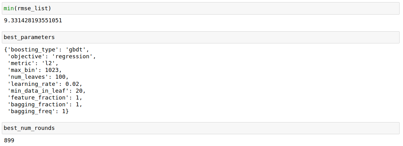
Again, we build this model 25 times on different random test-train splits (same code as in the “First test” part, but with best_parameters and best_num_rounds):

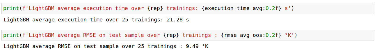
To give some perspective about this result, let us note that the standard deviation of the 25 RMSEs is approximately equal to 0.2. Their range is about 0.7.

Conclusion

In the end, our LightGBM model has achieved similar performance to XGBoost regarding both speed and accuracy. This does not mean that we could not reach better performance if we went deeper into hyperparameter tuning and grid searching. However, we can note that regarding this specific superconductivity problem/dataset, LightGBM did not trivially provided a better model than XGBoost. The source code of this experiment is entirely available on Github.

References

[1] HAMIDIEH, Kam A Data-Driven Statistical Model for Predicting the Critical Temperature of a Superconductor, University of Pennsylvania, Wharton, Statistics Department, 2018.

[2] CHEN, T., GUESTRIN, C. (2016). Xgboost: A scalable tree boosting system, University of Washington, 2016.

[3] Guolin Ke, Qi Meng, Thomas Finley, Taifeng Wang, Wei Chen, Weidong Ma, Qiwei Ye, Tie-Yan Liu. LightGBM: A Highly Efficient Gradient Boosting Decision Tree. Advances in Neural Information Processing Systems 30 (NIPS 2017), pp. 3149-3157.

See also

• Full Stack Data Engineering
• A multi container ML app (1/3): Docker
• An asymmetric loss for regression models
• Interpretable machine learning with SHAP
• Image recognition with PyTorch and fastai